Example Scripts

There are several ways to run XYmath

1. Launch the GUI, enter and fit data and perhaps run some math operations

   • (see Launch GUI and Entering Data and Math Operations)

2. Write a script to launch the GUI with data

3. Run a script that outputs to the console

The examples that follow will show both GUI and console scripts (options 2 & 3 above).

Warning

It is dangerous to run a console curve fit and accept it without looking at a plot.

Curve fitting is mostly about what happens Between the points, not At the points.

Instrument Calibration

This example comes from: http://terpconnect.umd.edu/~toh/spectrum/CurveFitting.html

The author shows a linear fit of an instrument reading chemical concentrations

The author mentions that a quadratic fit w/o the data point at concentration=0.6 would be significantly better… that is also calculated.

With GUI

The script /xymath/examples/calibration_gui.py launches the XYmath GUI with the calibration data so that the GUI can perform the desired calculations.

from numpy import array
from xymath.dataset import DataSet
from xymath.linfit import LinCurveFit
from xymath.xy_job import XY_Job
from xymath.gui.xygui import main as run_gui

concL = [0.1,0.2,0.3,0.4,0.5,0.6,0.7,0.8,0.9,1]
readingL = [1.54,2.03,3.17,3.67,4.89,6.73,6.74,7.87,8.86,10.35]
DS = DataSet(concL, readingL, xName='Concentration', yName='Instrument Reading')

XY = XY_Job()
XY.define_dataset(concL, readingL, wtArr=None, xName='Concentration',
                  yName='Instrument Reading', xUnits='', yUnits='')
run_gui( XY )

Once launched, the following steps can be taken inside the GUI:

1) Launch XYmath with code above
2) Go to "Simple Fit" Tab
3) Hit "Curve Fit"
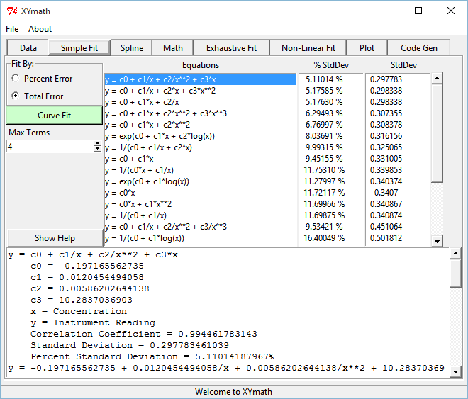
    - XYmath will show "c0 + c1/x + c2/x**2 + c3*x" as best fit
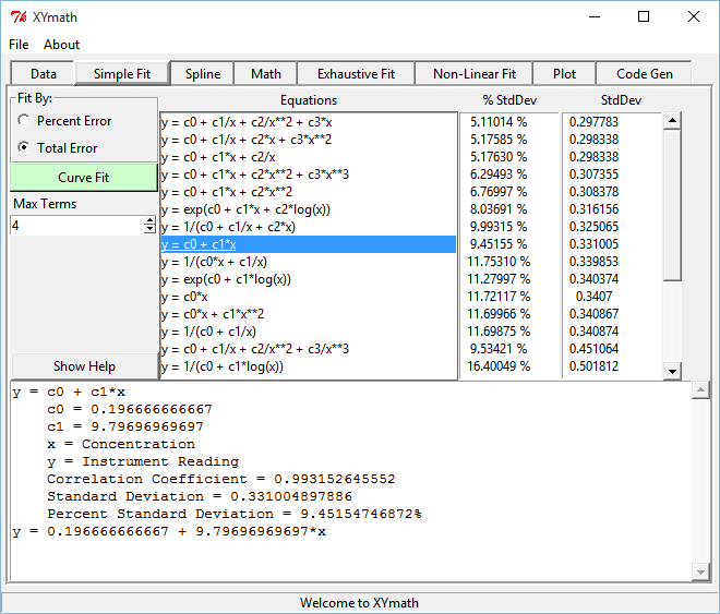
4) Select "y = c0 + c1*x" to approximate the author's results
5) Go to "Data" Tab
6) Select "weight" of data point with concentration=0.6
    - Set that weight to 0.0
7) Go back to "Simple Fit" Tab and hit "Curve Fit"
    - Notice that the zero-weighted point is marked as such on the plot
    - As the author predicts, the fit is greatly improved
    - Surprisingly, XYmath shows the 3 term equation "y = c0 + c1*x + c2/x"
      to be superior to the 4 term equations as well as the quadratic.

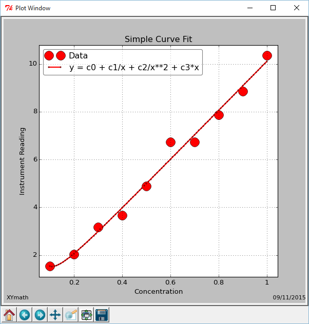
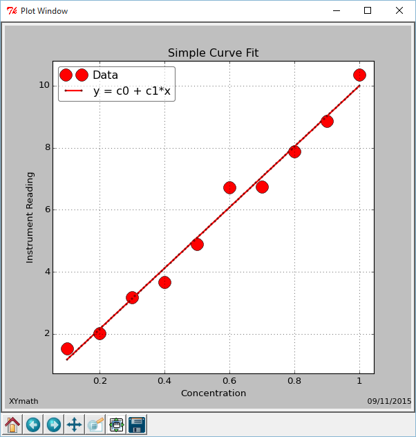
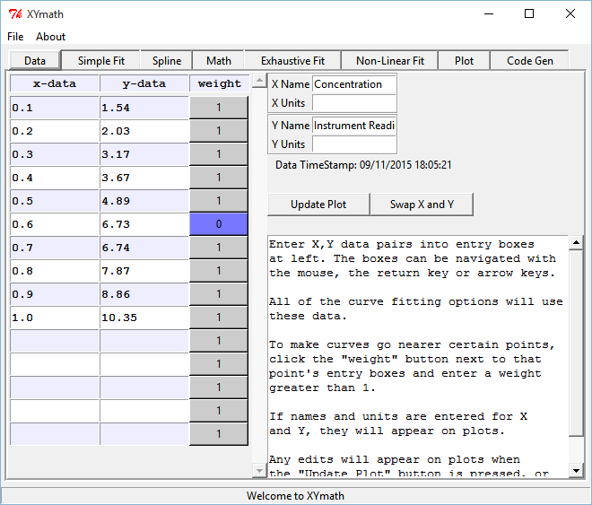
Running the above code, launches the GUI, preloaded with the concentration data.

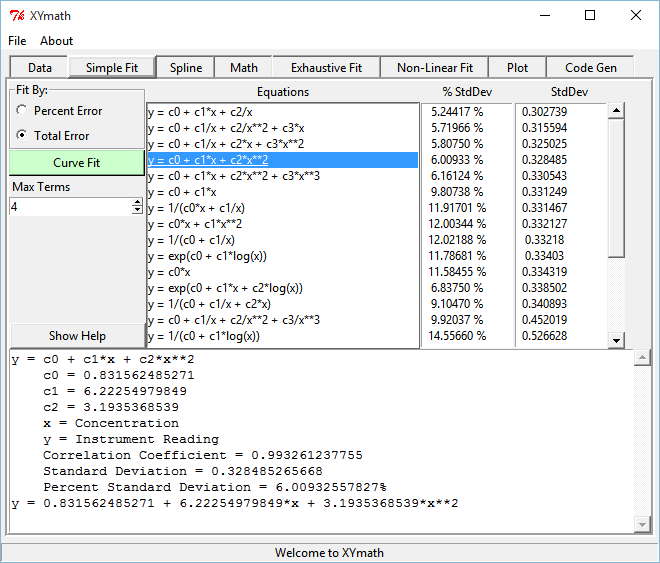
Using “Simple Fit” results in the GUI and plot shown below.

Selecting the straight line “y = c0 + c1*x” gives the GUI and plot shown below.

Use “Data” tab to set weight of data point at concentration=.6 to zero.

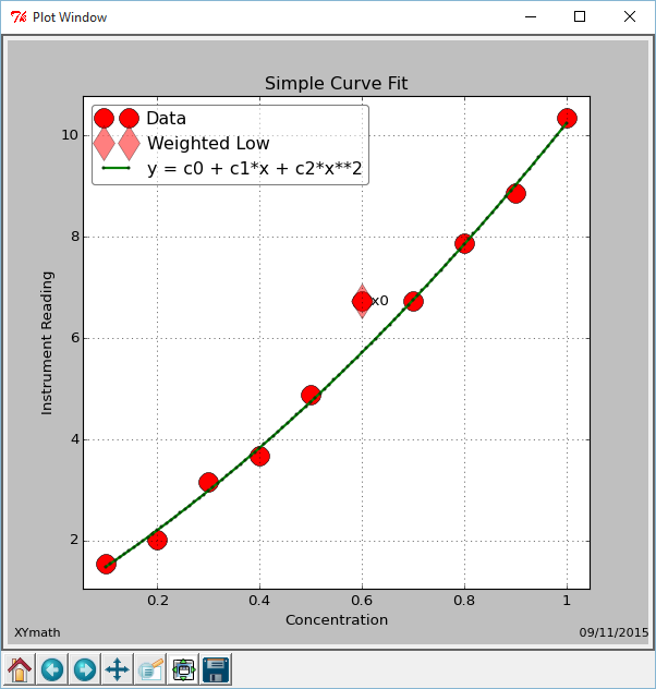
Rerun “Simple Fit” and select author’s quadratic recommendation

Notice that the data point at concentration=0.6 is still on the plot, but it is labeled as “Weighted Low” and its weight value is indicated as “x0”.

With Console

As you might imagine, the console script is longer because it performs many of the steps done manually in the GUI example.

This example first duplicates the author’s equation (i.e. sets the straight line coefficients to the same values as the author (cArrInp=[0.199, 9.7926]) and calculates standard deviation and percent standard deviation as a reference.

Then runs XYmath to fit the points. It results in only a very slight improvment in the author’s answer (see output below python script).

And finally removes the point at concentration=0.6 and fits to a quadratic. This results in the big improvement that the author was looking for (see output below python script).

Here’s the code from /xymath/examples/calibration.py.

try:
    from matplotlib import pyplot as plt
    got_plt = True
except:
    got_plt = False

from xymath.dataset import DataSet
from xymath.linfit import LinCurveFit

concL = [0.1,0.2,0.3,0.4,0.5,0.6,0.7,0.8,0.9,1]
readingL = [1.54,2.03,3.17,3.67,4.89,6.73,6.74,7.87,8.86,10.35]
DS = DataSet(concL, readingL, xName='Concentration', yName='Instrument Reading')

print('\n\n')
print('='*55)
print(".... First show author's answer ....")
Fit_ref = LinCurveFit(DS, xtranL=['const', 'x'] , ytran='y', cArrInp=[0.199, 9.7926],
                  fit_best_pcent=0)   # 0=fit best total error
print(Fit_ref.get_full_description())

print('='*55)
print('.... Then show XYmath answer ....')
Fit_linear = LinCurveFit(DS, xtranL=['const', 'x'] , ytran='y',
                  fit_best_pcent=0)   # 0=fit best total error
print(Fit_linear.get_full_description())

print('='*55)
print('.... Then show XYmath Quadratic answer ....')

v2_concL =    [0.1,  0.2, 0.3, 0.4, 0.5, 0.7, 0.8, 0.9, 1]
v2_readingL = [1.54,2.03,3.17,3.67,4.89,6.74,7.87,8.86,10.35]
DS = DataSet(v2_concL, v2_readingL, xName='Concentration', yName='Instrument Reading')

Fit_quad = LinCurveFit(DS, xtranL=['const', 'x', 'x**2'] , ytran='y',
                  fit_best_pcent=0)   # 0=fit best total error
print(Fit_quad.get_full_description())

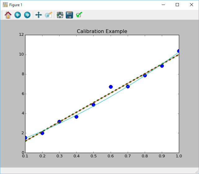
if got_plt:
    plt.plot( concL, readingL, 'o', markersize=10  )
    xPlotArr, yPlotArr = Fit_ref.get_xy_plot_arrays( Npoints=100, logScale=False)
    plt.plot( xPlotArr, yPlotArr, '--', linewidth=4  )
    xPlotArr, yPlotArr = Fit_linear.get_xy_plot_arrays( Npoints=100, logScale=False)
    plt.plot( xPlotArr, yPlotArr, '-'  )
    xPlotArr, yPlotArr = Fit_quad.get_xy_plot_arrays( Npoints=100, logScale=False)
    plt.plot( xPlotArr, yPlotArr, '-'  )
    plt.title('Calibration Example')
    plt.show()

The console output is shown below:

=======================================================
.... First show author's answer ....
y = c0 + c1*x
    c0 = 0.199
    c1 = 9.7926
    x = Concentration
    y = Instrument Reading
    Correlation Coefficient = 0.993152645552
    Standard Deviation = 0.331007277412
    Percent Standard Deviation = 9.42865864393%
y = 0.199 + 9.7926*x
=======================================================
.... Then show XYmath answer ....
y = c0 + c1*x
    c0 = 0.196666666667
    c1 = 9.79696969697
    x = Concentration
    y = Instrument Reading
    Correlation Coefficient = 0.993152645552
    Standard Deviation = 0.331004897886
    Percent Standard Deviation = 9.45154746872%
y = 0.196666666667 + 9.79696969697*x
=======================================================
.... Then show XYmath Quadratic answer ....
y = c0 + c1*x + c2*x**2
    c0 = 0.8315625
    c1 = 6.22254971591
    c2 = 3.19353693182
    x = Concentration
    y = Instrument Reading
    Correlation Coefficient = 0.999039190283
    Standard Deviation = 0.129698349765
    Percent Standard Deviation = 4.11221905227%
y = 0.8315625 + 6.22254971591*x + 3.19353693182*x**2

If matplotlib is installed on your machine, then you should see the following plot

Atmospheric Pressure

This example comes from: http://www.engineeringtoolbox.com/air-altitude-pressure-d_462.html

The author shows a non-linear fit of atmospheric pressure vs altitude.

The author derives a curve fit of air pressure above sea level as:

pressure(Pa)  = 101325 * (1 - 2.25577E-5 * h)**5.25588
where x=altitude(m)

With GUI

The script /xymath/examples/fit_Patmos_gui.py launches the XYmath GUI with the atmospheric data so that the GUI can perform the desired calculations.

from numpy import array, double
from xymath.xy_job import XY_Job
from xymath.gui.xygui import main as run_gui

XY = XY_Job()

alt_mArr = array([-1524,-1372,-1219,-1067,-914,-762,-610,-457,-305,-152,0,152,
           305,457,610,762,914,1067,1219,1372,1524,1829,2134,2438,2743,3048,4572,
           6096,7620,9144,10668,12192,13716,15240], dtype=double)

PaArr = 1000.0 * array([121,119,117,115,113,111,109,107,105,103,101,99.5,97.7,96,
        94.2,92.5,90.8,89.1,87.5,85.9,84.3,81.2,78.2,75.3,72.4,69.7,57.2,46.6,37.6,
        30.1,23.8,18.7,14.5,11.1], dtype=double)

XY.define_dataset(alt_mArr, PaArr, wtArr=None, xName='altitude', yName='Pressure',
                  xUnits='m', yUnits='Pa')


guessD = {'A':100000, 'c':1, 'd':0.00001, 'n':4  }

XY.fit_dataset_to_nonlinear_eqn(run_best_pcent=0, rhs_eqnStr='A*(c - d*x)**n',
                                constDinp=guessD)

run_gui( XY )

Once launched, the following steps can be taken inside the GUI:

1) Launch XYmath with code below
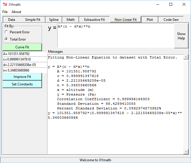
2) Go to "Non-Linear Fit" Tab
   - Should see "A*(c - d*x)**n" in eqn box
3) Hit "Curve Fit"

    y = A*(c - d*x)**n
        A = 101351.958792
        c = 0.999991347618
        d = 2.22155669208e-05
        n = 5.34803660866
        x = altitude (m)
        y = Pressure (Pa)
        Correlation Coefficient = 0.999996164903
        Standard Deviation = 88.4289410055
        Percent Standard Deviation = 0.0992974873982%

4) Change the "Fit By" flag to "Percent Error".
   Notice the XYmath improves Percent StdDev fit very slightly

    y = A*(c - d*x)**n
        A = 101124.977819
        c = 1.00041249485
        d = 2.23356723474e-05
        n = 5.31856523127
        x = altitude (m)
        y = Pressure (Pa)
        Correlation Coefficient = 0.999996135864
        Standard Deviation = 88.761441745
        Percent Standard Deviation = 0.094401748723%

Running the above code, launches the GUI, preloaded with the atmospheric data.

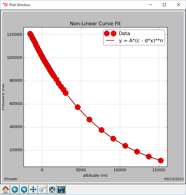
Using “Non-Linear Fit” results in the GUI and plot shown below.

With Console

Here’s the code from /xymath/examples/fit_Patmos.py. The code generates two curve fits, one with minimum total error and one with minimum percent error. The reference curve from www.engineeringtoolbox.com is also placed into a NonLinCurveFit object.

try:
    from matplotlib import pyplot as plt
    got_plt = True
except:
    got_plt = False

from numpy import array, double
from xymath.dataset import DataSet
from xymath.nonlinfit import NonLinCurveFit

alt_mArr = array([-1524,-1372,-1219,-1067,-914,-762,-610,-457,-305,-152,0,152,305,457,
          610,762,914,1067,1219,1372,1524,1829,2134,2438,2743,3048,4572,6096,7620,
          9144,10668,12192,13716,15240], dtype=double)

PaArr = 1000.0 * array([121,119,117,115,113,111,109,107,105,103,101,99.5,97.7,96,94.2,92.5,90.8,
        89.1,87.5,85.9,84.3,81.2,78.2,75.3,72.4,69.7,57.2,46.6,37.6,30.1,23.8,
        18.7,14.5,11.1], dtype=double)

DS = DataSet(alt_mArr, PaArr, xName='altitude', yName='pressure', xUnits='m', yUnits='Pa')


guessD = {'A':101325, 'c':1, 'd':2.25577E-5, 'n':5.25588  }
print( 'guessD Before',guessD )
CFit_toterr = NonLinCurveFit(DS, rhs_eqnStr='A*(c - d*x)**n',
                                constDinp=guessD, fit_best_pcent=0)   # 0=fit best total error
print( 'guessD After',guessD )

print('='*55)
print('..........Total Error............')
print(CFit_toterr.get_full_description())
print('='*55)
print('..........Percent Error............')
CFit_pcterr = NonLinCurveFit(DS, rhs_eqnStr='A*(c - d*x)**n',
                                constDinp=guessD, fit_best_pcent=1)   # 1=fit best percent error
print(CFit_pcterr.get_full_description())
print('='*55)

# To set parameters to reference values from www.engineeringtoolbox.com do this:
print('..........Reference Curve Fit............')
CFit_ref = NonLinCurveFit(DS, rhs_eqnStr='A*(c - d*x)**n', constDinp=guessD)
CFit_ref.constD.update( {'A':101325, 'c':1, 'd':2.25577E-5, 'n':5.25588  } )
CFit_ref.calc_std_values()
print(CFit_ref.get_full_description())

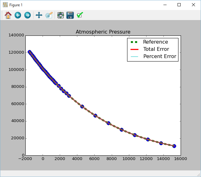
if got_plt:
    plt.plot( alt_mArr, PaArr, 'o', markersize=10  )
    xPlotArr, yPlotArr = CFit_ref.get_xy_plot_arrays( Npoints=100, logScale=False)
    plt.plot( xPlotArr, yPlotArr, '--', linewidth=5, label='Reference'  )
    xPlotArr, yPlotArr = CFit_toterr.get_xy_plot_arrays( Npoints=100, logScale=False)
    plt.plot( xPlotArr, yPlotArr, '-', label='Total Error' , linewidth=3 )
    xPlotArr, yPlotArr = CFit_pcterr.get_xy_plot_arrays( Npoints=100, logScale=False)
    plt.plot( xPlotArr, yPlotArr, '-', label='Percent Error'  )
    plt.title('Atmospheric Pressure')
    plt.legend()
    plt.show()

The console output is shown below

Note

After the curve fit, guessD holds the fitted values of the parameters.

('guessD Before', {'A': 101325, 'c': 1, 'd': 2.25577e-05, 'n': 5.25588})
('guessD After', {'A': 101071.99507528808, 'c': 1.0005086965155954, 'd': 2.2227059781416107e-05, 'n': 5.3480367230661061})
=======================================================
..........Total Error............
y = A*(c - d*x)**n
    A = 101071.995075
    c = 1.00050869652
    d = 2.22270597814e-05
    n = 5.34803672307
    x = altitude (m)
    y = pressure (Pa)
    Correlation Coefficient = 0.999996164903
    Standard Deviation = 88.4289426009
    Percent Standard Deviation = 0.0992975318388%
y = 101071.995075*(1.00050869652 - 2.22270597814e-05*x)**5.34803672307
=======================================================
..........Percent Error............
y = A*(c - d*x)**n
    A = 101749.173838
    c = 0.999255692815
    d = 2.2309845172e-05
    n = 5.31856519674
    x = altitude (m)
    y = pressure (Pa)
    Correlation Coefficient = 0.999996135864
    Standard Deviation = 88.7614426959
    Percent Standard Deviation = 0.0944017487367%
y = 101749.173838*(0.999255692815 - 2.2309845172e-05*x)**5.31856519674
=======================================================
..........Reference Curve Fit............
y = A*(c - d*x)**n
    A = 101325
    c = 1
    d = 2.25577e-05
    n = 5.25588
    x = altitude (m)
    y = pressure (Pa)
    Correlation Coefficient = 0.999995821319
    Standard Deviation = 93.2374437135
    Percent Standard Deviation = 0.106440180482%
y = 101325*(1 - 2.25577e-05*x)**5.25588

If matplotlib is installed on your machine, then you should see the following plot

Trigonometric Function

This example comes from: http://www.walkingrandomly.com/?p=5215

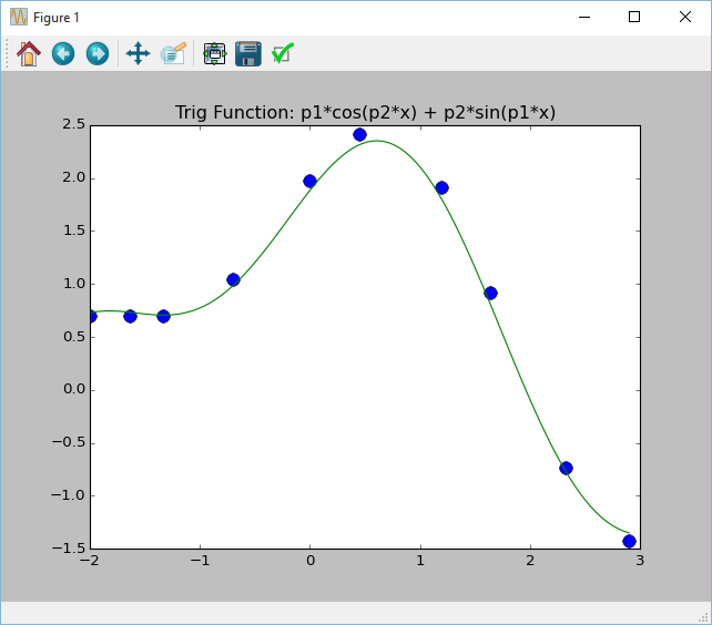
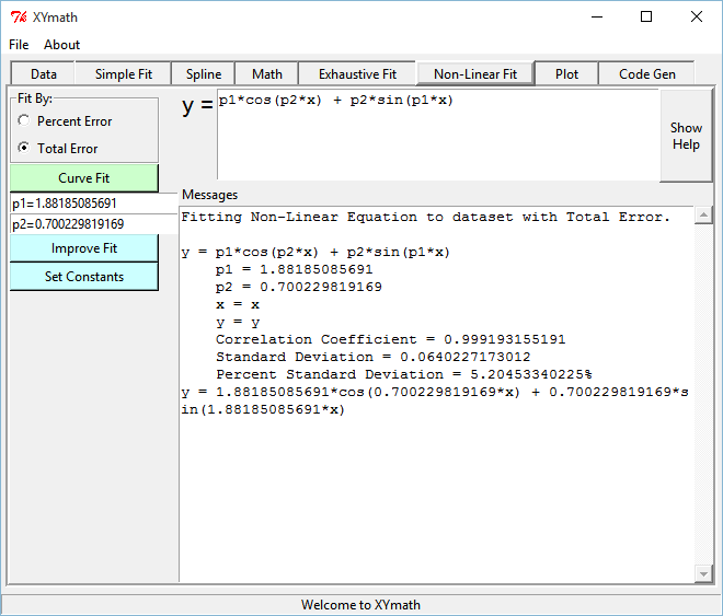
The author (Mike Croucher) wants to fit the equation:

y = p1*cos(p2*x) + p2*sin(p1*x)

to some (x,y) data.

He makes an initial guess of p1=1 and p2=0.2 and gets an answer of:

p1 = 1.88184732
p2 = 0.70022901

With no initial guess, XYmath gets very nearly the same answer:

p1 = 1.88185084847
p2 = 0.70022981688

With GUI

The script /xymath/examples/walking_randomly_gui.py launches the XYmath GUI with the trig function data so that the GUI can perform the desired calculations.

from xymath.xy_job import XY_Job
from xymath.gui.xygui import main as run_gui

XY = XY_Job()

xdata = [-2,-1.64,-1.33,-0.7,0,0.45,1.2,1.64,2.32,2.9]
ydata = [0.699369,0.700462,0.695354,1.03905,1.97389,2.41143,1.91091,0.919576,-0.730975,-1.42001]

XY.define_dataset(xdata, ydata, wtArr=None, xName='x', yName='y', xUnits='', yUnits='')

XY.fit_dataset_to_nonlinear_eqn(run_best_pcent=0, rhs_eqnStr='p1*cos(p2*x) + p2*sin(p1*x)')

run_gui( XY )

Once launched, the following steps can be taken inside the GUI:

1) Launch XYmath with code above
2) Go to "Non-Linear Fit" Tab
   - should see "p1*cos(p2*x) + p2*sin(p1*x)" in eqn box
3) Hit "Curve Fit"
4) See what happens when you hit "Improve Fit" a few times
5) Change to "Percent Error" and notice changes

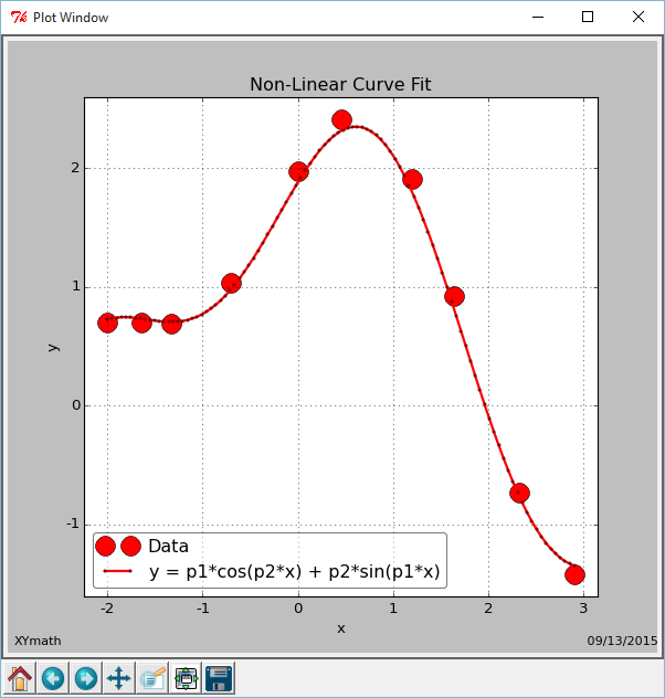
Running the above code, launches the GUI, preloaded with the trig function data.

Using “Non-Linear Fit” results in the GUI and plot shown below.

With Console

Here’s the code from /xymath/examples/walking_randomly.py. The code generates a curve fit of the equation ( y = p1*cos(p2*x) + p2*sin(p1*x) ).

try:
    from matplotlib import pyplot as plt
    got_plt = True
except:
    got_plt = False

from numpy import array
from xymath.dataset import DataSet
from xymath.nonlinfit import NonLinCurveFit

xdata = array([-2,-1.64,-1.33,-0.7,0,0.45,1.2,1.64,2.32,2.9])
ydata = array([0.699369,0.700462,0.695354,1.03905,1.97389,2.41143,
               1.91091,0.919576,-0.730975,-1.42001])
DS = DataSet(xdata, ydata, xName='x', yName='y')

guessD = {'p1':1.0, 'p2':0.2}
CFit = NonLinCurveFit(DS, rhs_eqnStr='p1*cos(p2*x) + p2*sin(p1*x)',
                      constDinp=guessD, fit_best_pcent=0)   # 0=fit best total error

print( 'residuals from XYmath = %g'%sum( (CFit.eval_xrange( xdata ) - ydata)**2 ) )
print( 'residuals from author = 0.053812696547933969' )
print('')
print(CFit.get_full_description())

if got_plt:
    plt.plot( xdata, ydata, 'o', markersize=10  )
    xPlotArr, yPlotArr = CFit.get_xy_plot_arrays( Npoints=100, logScale=False)
    plt.plot( xPlotArr, yPlotArr )
    plt.title('Trig Function: p1*cos(p2*x) + p2*sin(p1*x)')
    plt.show()

The console output is shown below:

residuals from XYmath = 0.0538127
residuals from author = 0.053812696547933969

y = p1*cos(p2*x) + p2*sin(p1*x)
    p1 = 1.881850994
    p2 = 0.700229857403
    x = x
    y = y
    Correlation Coefficient = 0.99919315158
    Standard Deviation = 0.0640227178858
    Percent Standard Deviation = 5.2045450232%
y = 1.881850994*cos(0.700229857403*x) + 0.700229857403*sin(1.881850994*x)

If matplotlib is installed on your machine, then you should see the following plot